Active Learning

When building supervised learning models, I often find myself working with data that falls into one of the following categories:

1. Labels are messy and/or innacurate
2. Dataset was never labeled in the first place

Obviously, it is not ideal to have to label every single datapoint, especially when there are thousands upon thousands of rows in your dataset.

I was recently tasked with building a sentiment analysis model for a dataset that fell into the second category. This dataset was quite domain-specific, which meant that the solution was more complicated than using a sentiment lexicon model like TextBlob or NLTK Vader. In this case, I found Active Learning to be quite useful for a few reasons:

• Active learning lets you start out with a small labeled subset of data
• Active learning allows you to diagnose where the model is struggling or confused, so that you can directly tell the model the correct answer
• Bulding on the last point, Active Learning allows you to intelligently label points, rather than making you go through the dataset aimlessly.

Here I’m going to show you a general breakdown of the active learning process.

Active Learning Process

Generally, active learning problems start out with a small labeled training set, and a really large set of unlabeled rows. We want to be able to leverage these unlabeled rows in a way that maximizes model performance given the least amount of time selecting examples from this unlabeled set.

At each iteration of the active learning process, you want to find the most ambiguous data points, label them, and then retrain the model with these labeled points. Selecting points that are near the decision boundary of the model will bolster it’s ability to descriminate between each class.

Selecting unlabeled points

There are a few different ways in which you can approach the selection process at each iteration. One of the more common ways is margin sampling. Imagine your model can predict either 0 or 1, and you have three points to predict. Now lets say the outputted probabilities are:

     Label Probability
           0    1
Point 1: [0.5, 0.5]
Point 2: [0.1, 0.9]
Point 3: [0.7, 0.3]

Here, The model is pretty confident about classifying Point 2 as 1. But look at Point 1. The model is basically making a guess here. It is not sure what category to choose. Cases like Point 1 are what we want to pull out of the unlabeled dataset and label ourselves, so that we can strengthen predictions near the decision boundary. Margin sampling simply finds all of the predictions that are closest to the decision boundary between two classes.

In python, we can calculate margin sampling with the following function:

def margin(probs):
    #First, sort columns in ascending order
    probs = np.sort(probs, axis = 1)
    #find the difference between the last and second-to-last probability
    diff = probs[:,-1] - probs[:,-2]
    #return sorted locations of differences
    idxs = np.argsort(diff)
    return idxs

Running margin() on our previous example will return something like

array([0, 2, 1], dtype=int64)

Since the model is the least confident about the first entry, and likewise most confident about the second entry.

Constructing an Active Learner

Now that we now how to select points to label at each step, we can start constructing a class that will help us train our model.

We first need to feed the class the labeled training data, as well as the unlabeled data. Also, we need to specify the model that we will be iteratively training. Finally, we will start by fitting the model to just the labeled data.

class ActiveLearner():
    def __init__(self, X_train, Y_train, unlabeled, model, sampler = 'margin'):
        self.sampler = eval("self.{}".format(sampler))
        self.X_train = X_train
        self.Y_train = Y_train
        self.label_set = np.unique(Y_train)
        self.unlabeled = np.array(unlabeled)
        self.model = model
        self.model.fit(self.X_train, self.Y_train)

For each step in the Active Learning process, we need to find the most confusing points.

def step(self, num_items):
    #get prediction probabilities for unlabeled data
    probas = self.model.predict_proba(self.unlabeled)
    #find most confusing points
    idxs = self.sampler(probas)
    #get top most confusing points
    top_idxs = idxs[:num_items]
    #return indexes and rows
    return top_idxs, self.unlabeled[top_idxs]

Now that we have used step() to find the most confusing points, we can provide the labels to these points and retrain the model.

def learn(self, data, target):
    #Add newly labeled points to X_train
    self.X_train = np.concatenate((self.X_train, np.array(data)))
    #Add new labels to Y_train
    self.Y_train = np.concatenate((self.Y_train, np.array(target)))
    #Refit model with new labels
    self.model.fit(self.X_train, self.Y_train)

But we haven’t given any labels to the model yet. The next function will allow us to do this by passing labels to the command line:

def train(self, num_items):
    #find most confusing points
    idxs, vals = self.step(num_items)
    #print confusing points to terminal
    for i, val in enumerate(vals):
        print(i + 1, '---', val)
    #begin process for entering labels into command line
    #contains some statements for making sure input is allowed
    while True:
        print('\n')
        labels = input('Enter Labels: ').split()
        if labels[0] == 'end':
            labels = []
            break
        if len(labels) != num_items:
            print('\nError: Number of provided labels does not match.')
            continue
        if not all(val.isnumeric() for val in labels):
            print('\nError: Labels must be numeric.')
            continue
        else:
            break
    if len(labels) == 0:
        pass

Active Learning on Yelp Dataset

Now that we’ve built the ActiveLearning class, we can test it out on a simple dataset. I’m going to be using the Yelp dataset from the UCI Machine Learning Repository.

For some simple preprocessing, we can use the following function:

import re
from string import punctuation

def clean(review):
    review = re.sub('[0-9]', '', review)
    review = "".join([c for c in review if c not in punctuation])
    return review.lower()

Now we load and clean the data.

import pandas as pd

data = pd.read_csv('data/yelp.txt', sep = '\t', header = None)
data.columns = ['text', 'label']
data['cleaned'] = [clean(review) for review in data.text]
X, y = data['cleaned'].values, data['label'].values

The dataset currently contains 1000 labeled rows. Now to demonstrate the usefulness of Active Learning, lets say that we only have access to 20% of these rows as an initial training set. We can simulate this scenario by doing the following:

from sklearn.model_selection import train_test_split

X_train, X_test, Y_train, Y_test = train_test_split(X, y, train_size = 0.2)
X_train.shape, X_test.shape

((200,), (800,))

Let’s now build our base model that we will later iteratively improve upon. We’re going to be using a simple TF-IDF vectorizer with Logistic Regression, both with default parameters.

from sklearn.linear_model import LogisticRegression
from sklearn.feature_extraction.text import TfidfVectorizer
from sklearn.pipeline import Pipeline

vectorizer = TfidfVectorizer()
logregmodel = LogisticRegression()

pipe_model = Pipeline([('vectorizer', vectorizer),
                       ('logreg', logregmodel)])

Now we can take some base metrics so that we can track later improvement in our model.

from sklearn.metrics import balanced_accuracy_score

base_preds = learner.model.predict(X_test).astype(int)
base_acc = balanced_accuracy_score(base_preds, Y_test)
print('Accuracy Before Active Learning: {}'.format(base_acc))

Accuracy Before Active Learning: 0.7113597246127367

Now let’s begin iteratively improving the model with the Active Learning class. We’re going to train the model for 5 iterations, presenting 10 new labels per iteration, totalling to 50 newly labeled points after the process is complete.

accs = []

iterations = 5
num_samples_per_iter = 10
for i in range(iterations):
    idxs = learner.train(num_samples_per_iter)
    #Remove sampled values from X_test and Y_test to calculate current test accuracy
    #Just for demonstration purposes. You wouldn't have access to the unknown labels in a real scenario
    curr_X_test = np.delete(X_test, idxs)
    curr_Y_test = np.delete(Y_test, idxs)
    #get current predictions and accuracy
    curr_preds = learner.model.predict(curr_X_test).astype(int)
    curr_acc = balanced_accuracy_score(curr_preds, curr_Y_test)
    print(curr_acc)
    accs.append(curr_acc)

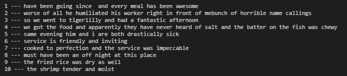
At each iteration, we come across a list of examples to be labeled:

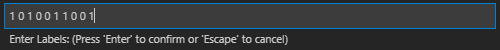
We can then enter the labels into the terminal as a list of integers:

Take a look at some of the examples we come across when training:

You can often tell right away when the model is struggling with certain vocabulary. In the above example, the model probably isn’t sure what “waited” means in the context of restaurant reviews.

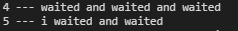
Below is another example that shows where the model is getting confused:

This is an ambiguous statement and seems positive at first, but is really holds a negative sentiment towards the target restaurant. It’s no wonder that a model as simple as this would be confused with such a statement.

Now that we’ve added 50 new labeled points, lets see how our model has improved over the course of training.

import matplotlib.pyplot as plt 

x_plot = np.arange(0, 60, 10)
plt.style.use('seaborn')
plt.figure(figsize=(12,6))
plt.plot(x_plot, [base_acc] + accs)
plt.xlabel('Number of Labeled Samples')
plt.ylabel('Balanced Accuracy')
plt.show()

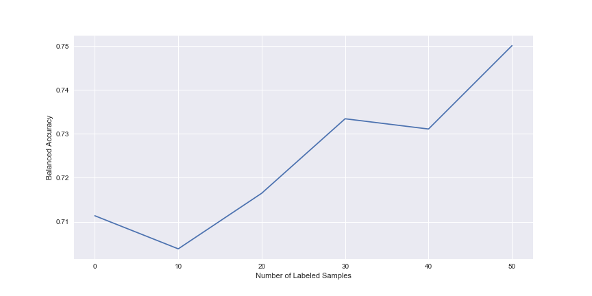
As you can see, model performance has increased to around 75% after only labeling 50 points. This is pretty good for just labeling 50 more points.

We can even compare our model after Active Learning with a model that simply used 50 extra randomly sampled datapoints. Let’s construct a second model in the exact same way as the first and see how it performs.

#sample 50 more datapoints randomly for train set
X_train_2, X_test_2, Y_train_2, Y_test_2 = train_test_split(X, y, train_size = 0.25, random_state = 2020)

second_pipe_model = Pipeline([('vectorizer', vectorizer),
                       ('logreg', logregmodel)])

second_pipe_model.fit(X_train_2, Y_train_2.astype(int))
second_preds = second_pipe_model.predict(X_test_2)
balanced_accuracy_score(second_preds, Y_test_2.astype(int))

0.7207772601794341

So here we see that the resulting accuracy from randomly sampling 50 more points ends up with worse overall balanced accuracy than when we had iteratively selected new points using Active Learning. Very interesting! Of course this isn’t an exhaustive comparison between both models. We would probably have to employ some sort of cross-validation if we wanted to be sure of the difference in performance. But this is interesting nonetheless.