Implementing and Exploring Naive Bayes for Text Classification

Background

Here, I’m going to be implementing Naive Bayes for the purposes of sentiment analysis.

My implementation largely relies on Chapter 4 of Speech and Language Processing by Jurafsky and Martin.

First we import some preliminary libraries for data structures and math/matrix operations.

import numpy as np
import pandas as pd

Dataset

I will be using three separate sentiment analysis datasets from here The combined dataset will consist of yelp restaurant reviews, IMDB movie reviews, and finally amazon product reviews. Hopefully this will give the model a holistic representation of the features that reveal the sentiment of a statement.

from nltk.stem.porter import PorterStemmer
from string import punctuation
from nltk.tokenize import word_tokenize
import nltk

data_names = ['amazon_cells_labelled.txt',
              'imdb_labelled.txt',
              'yelp_labelled.txt']
dataset = pd.DataFrame()

for name in data_names:
    df = pd.read_csv(name, sep = '\t', header = None)
    print(len(df))
    df.columns = ['Text', 'Label']
    dataset = pd.concat((dataset, df))

Now we clean the data. Pretty standard process. I’m going to first remove punctuation, then stem the words in hopes of reducing the dimensionality of the model while retaining semantic meaning.

stemmer = PorterStemmer()

def clean(text):
    lowered = text.lower()
    remove_punc = "".join([c for c in lowered if c not in punctuation])
    tokens =  word_tokenize(remove_punc)
    stemmed = [stemmer.stem(w) for w in tokens]
    return " ".join(stemmed)

cleaned = []
cleaned = [clean(text) for text in dataset['Text'].values]
cleaned = np.array(cleaned)
labels = dataset['Label'].values

Multinomial Naive Bayes

Now we can start to implement Naive Bayes for sentiment analysis. There are a few forms Naive Bayes can take on, depending on the type of input data your model is expecting. For example, Continuous input data utilizes Gaussian Naive Bayes, whereas categorical problems such as sentiment analysis and other text classification problems use Multinomial Naive Bayes. Further, we can even simplify the multinomial approach into a binary approach, as recommended by section 4.4 of Jurafsky and Martin.

Here is the Multinomial Naive Bayes algorithm to be implemented, taken directly from Chapter 4, page 6 of Jurafsky and Martin:

In order to convert this algorithm to the Binary case, we only need to consider the set of unique words in each sentence when building our log probabilities. In this sense, our model will only know if a word appeared in a sentence or not, rather than the amount of time a given word appears in each sentence.

Further, the Jurafsky and Martin implementation only considers the Add-One smoothing approach, but mentions that add-alpha smoothing should also be considered. I included this functionality to my implementation as well.

Building the Classifier

Now lets see how the model is implemented in python. First, we need to import another library.

from collections import Counter

Now we can begin to construct our class for Multinomial Naive Bayes. I tried as hard as I could to keep the same variable names as in the Jurafsky and Martin algorithm, so as to avoid confusion.

class multinomial_NB():
    def __init__(self, binary = False, alpha = 1):
        
        self.vocab = set()
        self.alpha = alpha
        self.C = []
        self.logprior = dict()
        self.loglikelihood = dict()
        self.bigdoc = dict()
        self.binary = binary
    
    #we need a function to create the vocab across all of the training data
    #In other words, this function creates 'V'
    
    def get_vocab(self, documents):
        vocab = set()
        for document in documents:
            for token in word_tokenize(document):
                vocab.add(token)
        return vocab
    
    def train(self, documents, labels):    
        self.vocab = self.get_vocab(documents)
        if self.binary == True:
            documents = np.array([" ".join(list(set(word_tokenize(doc)))) for doc in documents])
        self.C = np.unique(labels)
        for c in self.C:
            N_doc = len(documents)
            N_c = len(documents[labels == c])
            self.logprior[c] = np.log(N_c) -np.log(N_doc)
            self.bigdoc[c] = " ".join(documents[labels == c])
            tokens = word_tokenize(self.bigdoc[c])
            count = Counter(tokens)
            for word in self.vocab:
                self.loglikelihood[(word, c)] = np.log(count[word] + self.alpha)  - np.log(len(tokens)  + len(self.vocab))
    
    def predict(self, documents):
        predictions = []
        for document in documents:
            if self.binary == True:
                document = set(word_tokenize(document))
            else:
                document = word_tokenize(document)
            sums = []
            for c in self.C:
                sum_ = self.logprior[c]
                for w in document:
                    if w in self.vocab:
                        sum_ += self.loglikelihood[(w, c)]
                sums.append(sum_)
            predictions.append(np.argmax(sums))
        return predictions 

Validation

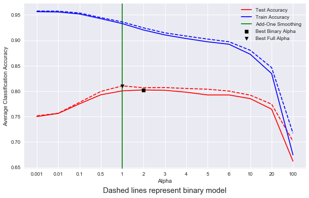
Now we can test our model. I’m going to use 10-fold cross validation in order to get a strong idea of the model’s final testing accuracy across different train/test splits. I am also interested in the effect of add-alpha smoothing on model performance, and so I’m going to create a trend-line across different values of alpha. Finally, both binary and full versions of the model will be cross-validated and compared to each-other across each value of alpha, to see what kind of performance changes arise when we only consider the binary case.

from sklearn.model_selection import KFold
from sklearn.metrics import accuracy_score

train_avgs = []
test_avgs = []

kf = KFold(n_splits = 10)
alphas = [0.001,0.01,0.1,.5,1,2,3,4,5,6,10,20,100]

for alpha in alphas:
    
    train_scores = []
    test_scores = []
    
    bin_train_scores = []
    bin_test_scores = []
    
    for train_index, test_index in kf.split(cleaned):
        X_train, X_test = cleaned[train_index], cleaned[test_index]
        Y_train, Y_test = labels[train_index], labels[test_index]
        
        #############regular model#############
        
        model = multinomial_NB(binary = False, alpha = alpha)
        model.train(X_train, Y_train)
        train_preds = model.predict(X_train)
        test_preds = model.predict(X_test)
        train_acc = accuracy_score(train_preds, Y_train)
        test_acc = accuracy_score(test_preds, Y_test)
        train_scores.append(train_acc)
        test_scores.append(test_acc)
        
        #############binary model##############
        binary_model = multinomial_NB(binary = True, alpha = alpha)
        binary_model.train(X_train, Y_train)
        train_preds = binary_model.predict(X_train)
        test_preds = binary_model.predict(X_test)
        train_acc = accuracy_score(train_preds, Y_train)
        test_acc = accuracy_score(test_preds, Y_test)
        bin_train_scores.append(train_acc)
        bin_test_scores.append(test_acc)
        
    
    train_avgs.append(np.mean(train_scores))
    test_avgs.append(np.mean(test_scores))
    bin_train_avgs.append(np.mean(bin_train_scores))
    bin_test_avgs.append(np.mean(bin_test_scores))
    
    print(bin_test_avgs[-1], test_avgs[-1])

751457199734572 0.7500066357000664
7565534173855342 0.756191108161911
7780172528201725 0.7751108161911082
799495686794957 0.7929502322495023
810406104844061 0.8005919044459191
8067657597876577 0.8024140676841407
8071293961512941 0.8016801592568015
8053125414731254 0.7980398142003982
8038553417385532 0.7925799601857996
80021499668215 0.7925799601857996
7922096881220969 0.7853005972130059
7743848706038488 0.7645587259455873
7016191108161911 0.6622959522229597

Visualization

Now let’s visualize the effect of our hyperparameter choices.

import matplotlib.pyplot as plt
plt.style.use('seaborn')

plt.figure(figsize = (10,6))

plt.plot(range(len(alphas)), test_avgs, 
         c = 'r', 
         label = 'Test Accuracy', 
         zorder = 1)

plt.plot(range(len(alphas)), bin_test_avgs, 
         c = 'r', 
         linestyle = '--',
         zorder = 1)

plt.plot(range(len(alphas)), train_avgs, 
         c = 'b', 
         label = 'Train Accuracy')

plt.plot(range(len(alphas)), bin_train_avgs, 
         c = 'b', 
         linestyle = '--')


plt.xticks(ticks = range(len(alphas)), labels = alphas)
plt.xlabel('Alpha')
plt.ylabel('Average Classification Accuracy')

best_alpha = np.argmax(test_avgs)
best_bin_alpha = np.argmax(bin_test_avgs)

plt.axvline(x=4.0, c = 'g', label = 'Add-One Smoothing', zorder = 1)

best_alpha = np.argmax(test_avgs)
best_bin_alpha = np.argmax(bin_test_avgs)

plt.scatter(best_alpha, test_avgs[best_alpha], 
            c = 'black', 
            marker = 's', 
            label = 'Best Binary Alpha', 
            alpha = 1, 
            zorder = 2)

plt.scatter(best_bin_alpha, 
            bin_test_avgs[best_bin_alpha], 
            c = 'black', 
            marker = 'v', 
            label = 'Best Full Alpha', 
            alpha = 1, 
            zorder = 2)
plt.text(6, .6, 
         'Dashed lines represent binary model', 
         ha = 'center', 
         fontdict = {'size': 15})

plt.legend()
plt.show()

Introducing N-grams

Let’s see if we can boost the performance of our model by introducing context windows. Currently, our model is using a bag-of-words approach, where word order does not matter. By introducing n-grams, perhaps we can build up dependencies between word-pairs such as “not good” and “didn’t like”. Since the order of tokens still doesn’t matter to a model like Naive Bayes, we can simply append these n-grams to the end of our original tokenized string. For example, with an n-gram window of (1,2), the following sentence:

This movie was not very good.

will be tokenized as

['this', 'movie', 'was', 'not', 'very', 'good', 'this movie', 'movie was', 'was not', 'not very', 'very good']

Likewise, for an n-gram window of (1,3), we would just add ‘this movie was’, ‘movie was not’, …

You get the idea.

Here is the updated multinomial_NB class with support for n-gram tokenization.

from nltk import bigrams

class multinomial_NB():
    def __init__(self, binary = False, alpha = 1, ngram_range = (1,)):
        self.vocab = set()
        self.ngram_range = ngram_range
        self.alpha = alpha
        self.C = []
        self.logprior = dict()
        self.loglikelihood = dict()
        self.bigdoc = dict()
        self.binary = binary
    
    def get_vocab(self, documents):
        vocab = set()
        for document in documents:
            tokens = []
            
            #iterate over each n-gram and extract tokens
            for ngram in self.ngram_range:
                tokens += list(nltk.ngrams(word_tokenize(document), ngram))
            for token in tokens:
                vocab.add(token)
        return vocab
    
    def tokenize(self, document, binary):
        tokens = []
        if self.binary == True:
            for ngram in self.ngram_range:
                tokens += list(set(nltk.ngrams(word_tokenize(document), ngram)))
        else:
            for ngram in self.ngram_range:
                tokens += list(nltk.ngrams(word_tokenize(document), ngram))
        return tokens
            
        
    def train(self, documents, labels):
        self.vocab = self.get_vocab(documents)
        
        if self.binary == True:
            tokenized = [self.tokenize(document, binary = True) for document in documents]
        else:
            tokenized = [self.tokenize(document, binary = False) for document in documents]
            
        self.C = np.unique(labels)
        for c in self.C:
            N_doc = len(documents)
            N_c = len(documents[labels == c])
            self.logprior[c] = np.log(N_c) -np.log(N_doc)
            self.bigdoc[c] = " ".join(documents[labels == c])
            tokens = []
            for ngram in self.ngram_range:
                tokens += list(nltk.ngrams(word_tokenize(self.bigdoc[c]), ngram))
            count = Counter(tokens)
            for token in self.vocab:
                self.loglikelihood[(token, c)] = np.log(count[token] + self.alpha)  - np.log(len(tokens)  + len(self.vocab))
    
    def predict(self, documents):
        predictions = []
        tokenized_docs = []
        if self.binary == True:
            for i, document in enumerate(documents):
                tokens = self.tokenize(document, binary = True)
                tokenized_docs.append(tokens)
        else:
            for i, document in enumerate(documents):
                tokens = self.tokenize(document, binary = False)
                tokenized_docs.append(tokens)
        documents = tokenized_docs        
        for document in documents:    
            sums = []
            for c in self.C:
                sum_ = self.logprior[c]
                for w in document:
                    if w in self.vocab:
                        sum_ += self.loglikelihood[(w, c)]
                sums.append(sum_)
            predictions.append(np.argmax(sums))
        return predictions

Notice how, in the code above, not much was changed, accept for one simple addition. Instead of using singular tokens to construct our vocabulary, we are going a step further and iterating over all n-grams defined in the ngram-range variable, and adding these additional tokens to our vocabulary.

This has an immense difference on the resulting size of our vocabulary. Let’s first observe what the original vocabulary size was when we used not context window:

model = multinomial_NB(gram_range = (1,))
model.train(X_train, Y_train)
print(len(model.vocab))

Now lets construct the vocabulary with an n-gram range of (1,2):

model = multinomial_NB(gram_range = (1,2))
model.train(X_train, Y_train)
print(len(model.vocab))

Which returns the following output:

Likewise, increasing the n-gram range to (1,2,3):

model = multinomial_NB(ngram_range = (1,2,3))
model.train(X_train, Y_train)
print(len(model.vocab))

gives us the following vocab size:

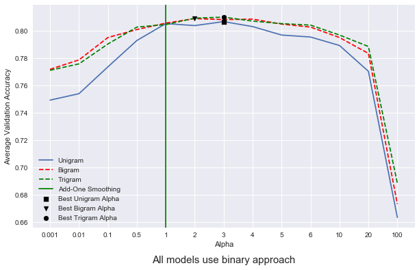
But does the introduction of n-grams improve model performance? Let’s explore the use the same cross-validated approach as above to compare unigram vs bigram vs trigram word-context configurations.

Here is the code for training each separate model.

uni_avgs = []
bigram_avgs = []

kf = KFold(n_splits = 10)
alphas = [0.001, 0.01, 0.1,.5, 1,2,3,4,5,6,10,20,100]

for alpha in alphas:
    uni_scores = []
    bi_scores = []
    tri_scores = []
    
    for train_index, test_index in kf.split(cleaned):
        X_train, X_test = cleaned[train_index], cleaned[test_index]
        Y_train, Y_test = labels[train_index], labels[test_index]
        
        ##########Unigram Model##############
        regular_model = multinomial_NB(binary = True, ngram_range = (1,), alpha = alpha)
        regular_model.train(X_train, Y_train)
        uni_preds = regular_model.predict(X_test)
        uni_scores.append(accuracy_score(uni_preds, Y_test))
        
        ###########Bigram Model##############
        bi_model = multinomial_NB(binary = True, ngram_range = (1,2), alpha = alpha)
        bi_model.train(X_train, Y_train)
        bi_preds = bi_model.predict(X_test)
        bi_scores.append(accuracy_score(bi_preds, Y_test))
        
        ##########Trigram Model##############
        tri_model = multinomial_NB(binary = True, ngram_range = (1,2,3), alpha = alpha)
        tri_model.train(X_train, Y_train)
        tri_preds = tri_model.predict(X_test)
        tri_scores.append(accuracy_score(tri_preds, Y_test))
        
    
    uni_avgs.append(np.mean(uni_scores))
    bigram_avgs.append(np.mean(bi_scores))
    tri_avgs.append(np.mean(tri_scores))

Now that each model has been trained, let’s plot our results.

plt.figure(figsize = (10,6))

plt.plot(uni_avgs, label = 'Unigram', zorder = 1)
plt.plot(bigram_avgs, label = 'Bigram', zorder = 1, linestyle = '--', c = 'r')
plt.plot(tri_avgs, label = 'Trigram', zorder = 1, c = 'g')

plt.ylabel('Average Validation Accuracy')
plt.xlabel('Alpha')
plt.xticks(ticks = range(len(alphas)), labels = alphas)

best_uni_alpha = np.argmax(uni_avgs)
best_bi_alpha = np.argmax(bigram_avgs)
best_tri_alpha = np.argmax(tri_avgs)

plt.axvline(x=4.0, c = 'g', label = 'Add-One Smoothing', zorder = 1)


plt.scatter(best_uni_alpha, uni_avgs[best_uni_alpha], 
            c = 'black', 
            marker = 's', 
            label = 'Best Unigram Alpha', 
            alpha = 1, 
            zorder = 2)

plt.scatter(best_bi_alpha, 
            bigram_avgs[best_bi_alpha], 
            c = 'black', 
            marker = 'v', 
            label = 'Best Bigram Alpha', 
            alpha = 1, 
            zorder = 2)

plt.scatter(best_tri_alpha, tri_avgs[best_tri_alpha],
            c = 'black',
            marker = 'o',
            label = 'Best Trigram Alpha',
            alpha = 1,
            zorder = 2)

plt.text(6, .63, 
         'All models use binary approach', 
         ha = 'center', 
         fontdict = {'size': 15})

plt.legend()
plt.show()

Discussion

We can see from our results that our choice of alpha does have a significant effect on the final test accuracy of our model. I picked some pretty arbitrary values for alpha, since the model takes quite a while to train when cross-validated 10 times, but it appears that the model performs well with an alpha set between the two extremes. Give too little probability to a word that is not seen in the training set and the model assigns innacurately low probabilities to sentences that contain too many words that aren’t in the training vocabulary. Likewise, giving too much probability to words that the model hasn’t seen seems to muddy the waters. In other words, having too many instances with high probabilities seems to force the model to make an uninformed guess on which class the data point should be assigned to.