Background
This was a project I created for UCSD’s CSE 156 (Statistical NLP). I’ve always been very interested in Sentiment Analysis and its applications, and so I decided to build a hate speech classifier using a GRU, as well as visualize the results.
GRU Architecture
First we import some keras dependencies.
from keras.models import Sequential
from keras.layers import Dense, Dropout, GRU
from keras.layers.embeddings import Embedding
from keras.preprocessing import sequence
Then we compile the keras model.
embedding_vector_length = 128
model = Sequential()
model.add(Embedding(vocab_size + 1, embedding_vector_length, input_length = 1000))
model.add(GRU(128))
model.add(Dropout(0.2))
model.add(Dense(1, activation = 'sigmoid'))
model.compile(loss = 'binary_crossentropy', optimizer = 'adam', metrics = ['accuracy'])
Training the model
Now we can start training our GRU
model.fit(X_train, y_train, validation_data = (X_val, y_val), epochs = 1, batch_size = 128)
806/806 [==============================] - 3s 4ms/step
Accuracy  80.769231%
And finally we can save our model to a json file for later use.
modeljson = model.to_json()
with open('model.json', 'w') as json_file:
    json_file.write(modeljson)
model.save_weights('model.h5')
Visualizing Hate Speech
from sklearn.metrics import pairwise_distances
from scipy.spatial.distance import cosine
Earlier, we trained our GRU with the idea of creating relationships between words in our dataset. Now, we can use the final hidden layer of our GRU as a basis for our trained word vectors.
vecs = model.layers[0].get_weights()[0]
word_embeds = {w:vecs[idx] for w, idx in vocab_to_int.items()}
Now we can represent the pairwise similarity of our word vectors using cosine distances.
cosines = 1 - pairwise_distances(vecs, metric = 'cosine')
cosines.shape
(16925, 16925)
Now lets create a function for finding the top k closest words based on cosine similarity.
def find_closest(word, num = 10):
    w1idx = vocab_to_int[word]
    sims = enumerate(cosines[w1idx,:])
    sorted_sims = sorted(sims, key = lambda x: x[1], reverse = True)
    sorted_sims = [sim for sim in sorted_sims if sim[0] != w1idx]
    words = [int_to_vocab[sim[0]] for sim in sorted_sims][:num]
    return words
Now we can create our clusters for visualization. First, we’re going to create a key that represents the center of each cluster. Then, we’re going to find the most similar words to each key as a representation for our clusters.
My keys contain a few common slurs I came across while browsing the dataset, as well as some neutral words like “white”, “black”, “twitter”, “facebook”, and “book”. I have censored the slurs.
keys = ['n*****', 'q****', 'f**', 'white', 'black', 'w******', 'c****', 'b*****', 'c***', 'twitter', 'facebook', 'book']
Now, we can start generating our clusters.
embedding_clusters = []
word_clusters = []
for word in keys:
    most_similar_words = find_closest(word, 100)
    embeddings = np.array([word_embeds[w2] for w2 in most_similar_words])
    embedding_clusters.append(embeddings)
    word_clusters.append(most_similar_words)
Now let’s see the shape of our clusters:
np.array(embedding_clusters).shape
(12, 100, 128)
The first index refers to how many clusters we have created. The second index refers to the top-k most similar words we found per key. The final index refers to the embedding dimension of each word vector.
Now, let’s plot the clusters. First are going to squash the word-embeddings down to two dimensions using TSNE in order to visualize the resulting clusters.
from sklearn.manifold import TSNE
embedding_clusters = np.array(embedding_clusters)
n, m, k = embedding_clusters.shape
tsne_model_2d = TSNE(perplexity = 15, n_components = 2, init = 'pca', n_iter = 3500)
embeddings_2d = np.array(tsne_model_2d.fit_transform(embedding_clusters.reshape(n * m, k))).reshape(n, m, 2)
And now that we have 2D representations of each cluster, we can start plotting.
import matplotlib.cm as cm
from profanity_check import predict as prof_pred # these are for censoring words in the resulting plot
from profanity_check import predict_prob
Here’s a function for plotting our clusters:
def tsne_plot_similar_words(labels, embedding_clusters, word_clusters, a):
    plt.figure(figsize = (16,9))
    colors = cm.rainbow(np.linspace(0,1,len(labels)))
    for label, embeddings, words, color in zip(labels, embedding_clusters, word_clusters, colors):
        x = embeddings[:,0]
        y = embeddings[:,1]
        if label in hate_words or prof_pred([label]) == 1:
            label = label[0] + '*'*(len(label) - 1)
            plt.scatter(x,y, c = 'r', alpha = a, label = label)
            for i, word in enumerate(words):
                if prof_pred([word]) == 1 or word in hate_words:
                    word = word[0] + '*'*(len(word) - 1)
                plt.annotate(word, alpha = 0.5, xy = (x[i], y[i]), xytext = (5,2),
                            textcoords = 'offset points', ha = 'right', va = 'bottom', size = 8)
        else:
            plt.scatter(x,y, c = 'b', alpha = a, label = label)
            for i, word in enumerate(words):
                if prof_pred([word]) == 1 or word in hate_words:
                    word = word[0] + '*'*(len(word) - 1)
                plt.annotate(word, alpha = 0.5, xy = (x[i], y[i]), xytext = (5,2),
                            textcoords = 'offset points', ha = 'right', va = 'bottom', size = 8)
    plt.legend(loc = 4)
    plt.grid(True)
And now we finally come across an interesting visualization like this:
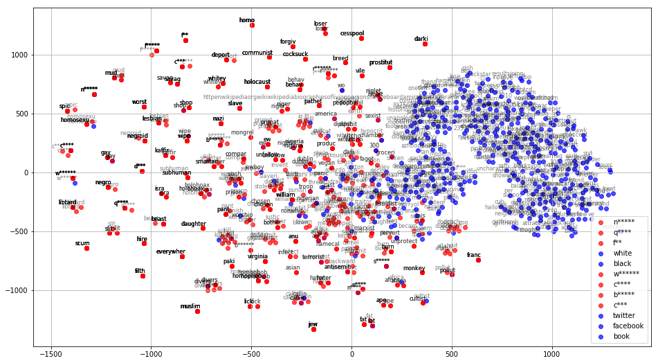
We can immediately see that the clusters referring to very neutral words like “twitter” and “facebook” are quite distanced from hate speech words. On the other hand, we also see that words like “white” and “black” are positioned very closely to our hate speech clusters. This is likely because words like “white” and “black” are used in both negative and positive contexts quite frequently.
If you want to play around with the visualizer yourself, I wrote a python script that allows you to enter your own keys and visualize the resulting clusters! I also wrote another script that allows you to use the classifier on your own entered text. You can view the master jupyter notebook file here. Finally, the repo to the entire project is linked right here.